<3

The biggest challenge of Bayesian Statistics lies in model inference, where one combines the prior and likelihood to derive a posterior. Most of the time, the posterior will not have an analytic form and so we have to rely on sampling methods such as MCMC. However, MCMC can be very computationally expensive, and in the age of big data, there is a lot of attention being directed towards developing new inference algorithms that could scale well to large datasets. In the last couple of years, Variational Inference has become a viable and scaleable alternative to MCMC for performing inference on complex Bayesian models. In this post, I’ll present the basic math underlying the mechanics of Variational Inference, and also present it in its most simple form: Coordinate Ascent Variational Inference. I’ll end with a practical example, showing how to apply Coordinate Ascent Variational Inference to a Mixture of Gaussians model. My derivations will be following (Blei 2016) very closely.

1. Introduction and the Problem
2. Statement of the objective
3. The ELBO
4. The mean field assumption and coordinate ascent
5. Example: Mixture of Gaussians

Introduction and the Problem

Recall Bayes rule, which gives us the procedure for drawing inferences from data:

The term in the denominator is often referred to as the marginal likelihood, or the evidence, and is what causes inference to be intractable. This is because to calculate \(p(D) \), we have to integrate over the space of all parameters: \(p(D) = \int_{\theta \in \Theta} p(D \vert \theta)p(\theta) \). Now if \(\theta \) is one dimensional this could work, but as the dimensionality of our parameter space increases, the number of computations needed also increases exponentially, making this an unfeasible numerical computation.

Variational Inference, or VI, belongs to a class of inference algorithms referred to as approximate inference, which is designed to get around this problem in a different way from MCMC. The idea is that instead of drawing samples from the exact posterior, such as MCMC, you instead approximate the posterior, trading off a little bit of bias in exchange for computational tractability. As such, these approximate inference methods transform inference from a sampling problem into an optimization problem, which is typically much more tractable and easier to deal with. VI is just one of the approximate inference algorithms, but it has been the one that has seen the most success and has been the most widely adopted.

Statement of the objective

Like previously stated, VI transforms inference from a sampling problem into a optimization problem. It does this by approximating the posterior \(p(\theta \vert x) \) with some class of distributions Q parameterized by what we call “variational parameters” \(\xi \). Note that the dimension of \(\xi \) depends on what variational distribution we choose. Then, we want to find \(\xi \) such that our variational distribution \(q(\theta \vert \xi)\) is “close” to the posterior. I’ll go ahead and note here that technically, our variational distribution is a function of x; the exact notation should probably be \(q(\theta \vert \xi(x) \)), but you’ll often see \(q(\theta) \text{ or } q(\theta \vert \xi) \) for brevity. Going back to the problem of defining “closeness”, the canonical measure that is used is the KL Divergence. Recall that for two distributions p, q, the KL divergence is defined as:

Our objective then becomes

And then once we have found \(q^{*}(\theta) \), we we use that as our approximate posterior. Again, I’ll stress that theres an implicit \(\xi \) that parameterizes our distribution q; so when I say to find the distribution that maximizes this quantity, I really mean find \(\xi \) that maximizes \(KL(q(\theta \vert \xi) \vert\vert p(\theta \vert x)) \).

However, we run into a big problem when we actually try and optimize this objective. Lets go ahead expand out the definition of the KL divergence:

We can see that the undesirable term, \(p(x) \) pops up again in this equation. Thus we have that the KL divergence is intractable and useless to us.

What can we do from here? The way forward is to note that since \(p(x) \) is a constant with respect to theta, we can drop it from the whole term and minimize the KL divergence up to an additive constant.

The ELBO

Define the Evidence Lower Bound (ELBO) as

Where the expectations are taken with respect to q. It might seem a bit weird to be taking the expectation of a distribution \(p(\mathbf{theta}, x)\), but here its just easier to think of \( p(\mathbf{\theta}, x)\) as some function of \(\theta \) with x held fixed.

Immeditely, we can see that the EBLO is simply the negative KL divergence plus some additive constant. Thus, maximizing the ELBO will minimize the KL divergence, which will then give us the variational distribution that we want. Furthermore, because we have dropped the intractable constant, we can actually compute the ELBO.

In addition to being our optimizational objective, the ELBO also has the nice property of providing a lower bound for the marginal likelihood/evidence (hence the name). To see this, observe that

Here, the above inequality followed from application of Jensen’s inequality.

Thus, we have formulated a tractable variational objective: find the distribution \(q(\theta \vert \xi) \in Q \) that maximizes the ELBO, which will in turn minimize the KL divergence between \(q \) and the posterior.

The Mean Field Assumption and the Coordinate Ascent Updates

Now that we have the function we want to maximize, the next step is to figure out how to actually maximize this thing. The easiest, and arguably simplest way, is to apply coordinate ascent, where we maximize with respect to one variable at each sweep, holding all others constant. Lets start by clarifying my notation. Let \(\theta \) be the vector of all parameters, and \(\theta_{j} \) be the jth parameter in the parameter vector. Similarly, let \(\mathbf{x} \) be the vector of observed data and \(x_{i} \) be the ith datapoint. Let \(-j \) denote everything except for j. For example, \(\mathbb{E}_{-j} [\mathbf{ \theta_{-j}}]\) would represent the expectation of all of the theta parameters, except for the jth one.

First, we make a simplifying assumption. In what we call the mean field assumption, we assume that the joint variational distributions of our parameters decomposes into the product of the marginals:

As we will see, this simplifies the derivations greatly. However, at the same time, it also completely ignores the covariance between the parameters, which is often why VI significantly underestimates the variance of its estimated parameters. This drawback is something to be aware of when choosing to make the mean field assumption or not.

Lets go ahead and manually maximize the ELBO. I claim that the optimal update for the variational distribution of \(q(\theta_{i}) \) takes the form

Where the expectation is taken with respect to the variational distributions of the parameters (the \(q\)’s). Note that we can rewrite the term in the expectation in a bunch of different ways: this is because \(p(\theta_{j} \vert \theta_{-j}, \mathbf{x}) \propto p(\theta_{j}, \theta_{-j} \vert \mathbf{x}) \propto p(\theta_{j}, \theta_{-j}, \mathbf{x})\) and so on. And, because it is a proportionality symbol, this is not a true distribution, but rather something that is proportional to a probability distribution, meaning that we have to re-normalize the variational distribution after computing this.

To prove that this really is the optimal update, begin by rewriting the ELBO as a function of \(\theta_{j} \):

To clarify, the first expectation is a k dimensional integral, since we have k parameters. I’m going to go ahead and apply iterated expectation to our first term, which then turns into

Expand the inner term \(\mathbb{E}_{-j}[\log\, p(\theta_{-j}, \theta_{j}, \mathbf{x}) \vert \theta_{-j}] = \int q(z_{-j} \vert z_{j})(\log\, p(\theta_{j}, \theta_{-j}, \mathbf{x})) = \int q(z_{-j})\log\, p(\theta_{j}, \theta_{-j}, \mathbf{x})\) where the last step followed because of our mean field assumption. Thus, the ELBO becomes

We can see that this takes the form of the negative KL Divergence between \(q(\theta_{j})\) and \(\exp(\mathbb{E}_{-j}[\log \, p(\theta_{j}, \theta_{-j}, \mathbf{x})]) = q^{*}(\theta)\) plus some additive constant. Thus, we maximize the ELBO when we minimize the above equation: ie. when we set \(q(\theta_{j}) = q^{*}(\theta_{j}) \).

Lets now step back and recap our algorithm. At each iteration, we want to set the variational distribution proportional to \(\exp(\mathbb{E}_{-j}[\log\, p(\theta_{j}, \theta_{-j}, \mathbf{x}))\). Then, calculate the ELBO \(\mathbb{E}[\log\, p(\theta,x)] - \mathbb{E}[\log\, q(\theta)]\). Repeat until convergence.

Now that we’ve gone through the mechanics of how Coordinate Ascent Variational Inference works, lets go ahead and see an example.

Example: Mixture of Gaussians

Consider a classic mixture model with K components, that has this setup:

The first step is to determine which variational distributions we place on each of the parameters. I’m going to go with a normal variational distribution for the component means, and a categorical distribution for the cluster assignments.

Putting it explicitly, we have

Note that the variational distributions do not have to be the same as the prior distributions; I could have picked any distribution I wanted to be the variational distribution. In practice however, its a good idea to have the support of your variational distribution and parameter space line up. As you can see above, the variational parameters to optimize are going to be the mean and variance of the normal variational distribution, and the probability vectors for the categorical distribution.

Lets start by deriving the update equations for \(c\) first. We have that for the ith cluster assignment (corresponding to the ith person), the joint distribution can be factorized as follows:

Where in the last step we have removed all of the terms that do not depend on i. Therefore, the update rule becomes

Recall that the expectation is taken with respect to everything except for the ith component - in this case, all of the mixture means. Obviously its taken with respect to the other cluster assignments too, but this is a constant with respect to that and so those terms in the expectation fall away.

Lets focus in on that expectation term. The key fact here, is noting that \(p(x_{k} \vert \mu, c_{i}) = \prod_{i=1}^{K}p(x_{i} \vert \mu_{i})^{c_{ik}}\). Thus, this becomes

I’m going to stress again that the expectations here are with respect to the variational distribution of \(\mu_{k}\); that is, a normal with mean m and variance \(s^{2}\). Thus, \(\mathbb{E}[\mu_{k}] = m, \mathbb{E}[\mu_{k}^{2}] = s^{2} + m^{2}\). When we put this expectation back into the update equation, we find that

If we stare at this long enough, we can notice that this is actually the exponential family representation for the multinomial, with natural parameter \(\eta_{k} = \log\, p_{k}= \log \exp( [m_{k}x_{i} - (m_{i}^2 + s_{i}^2)/2])) \). This implies that the optimal parameter value is given by \( \phi_{ik} \propto \exp(m_{k}x_{i} - (m_{i}^2 + s_{i}^2)/2)\). Note that we still have to normalize this, to enforce the constraints that\(\sum_{k} \phi_{ik} = 1 \).

Then, we’ll derive the updates for the means.

Our update is

Again, lets stare at this thing. We can again see that this is precisely the exponential family representation of a gaussian! This brings up an interesting question: does this result hold in general? Very interesting question indeed …

We can see from the above equation that the natural parameters are \(\eta_{1} = \sum_{i}\phi_{ik}x_{i}, \; \eta_{2} = -\frac{1}{2\sigma^2} - \sum_{i}\frac{\phi_{ik}}{2}\). Furthermore, recall that the mean parameterization of a normal is given by \(\mu = -\frac{\eta_{1}}{\eta_{2}}, \; \sigma^{2} = -\frac{1}{\eta_{2}}\). From this, we derive the parameters of our optimal variational distribution as

Now, the final step is to derive the ELBO. Generally, its a good idea to derive the ELBO first, but I decided to put it at the end, because once we have all of the component pieces, its only a matter of combining them to reproduce the ELBO.

We have that \(ELBO = \mathbb{E}[\log\, p(\mathbf{x},\mu,c)] - \mathbb{E}[\log\, q(\mu, c)]\). Lets expand out the first term:

As for the second term, we have:

Putting it together, we have:

And finally, we are done with our derivation. For me at least, this topic was something that I had to stew on for a while before I truly began to understand it. Going over the math and attempting to re-derive all of the update equations myself helped a lot with my comfort with the topic.

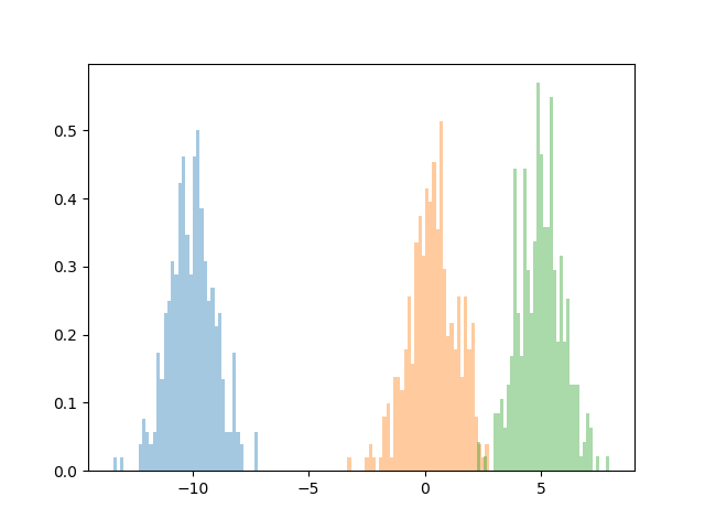
Now, lets go ahead and see an implementation of our algorithm. First, we’ll generate some data.

	import torch
	import torch.distributions
	import matplotlib as plt
	import seaborn as sns

	datapoints = torch.zeros(1000)
	datapoints[0:333] = torch.distributions.Normal(-10, 1).sample((333,))
	datapoints[333:666] = torch.distributions.Normal(.25, 1).sample((333,))
	datapoints[666:] = torch.distributions.Normal(5, 1).sample((333,))
	sns.distplot(list(datapoints[0:333]), kde=False, bins=50, norm_hist=True)
	sns.distplot(list(datapoints[333:666]), kde=False, bins=50, norm_hist=True)
	sns.distplot(list(datapoints[666:]), kde=False, bins=50, norm_hist=True)
	plt.show()

And here is the code to fit the mixture model, which implements the equations specified above:

	
	import torch
	import torch.distributions

	"""
	phi: K x N matrix of cluster assignments
	mu: K x 1 vector of cluster means
	x: N x 1 vector of data points
	"""

	def update_phi(m, s2, x):
		"""
		Variational update for the mixture assignments c_i
		"""
		a = torch.ger(x, m)
		b = (s2+m**2)*.5
		return torch.transpose(torch.exp(a-b), 0, 1)/torch.exp(a-b).sum(dim = 1)

	def update_m(x, phi, sigma_sq):
		"""
		Variational update for the mean of the mixture mean
		distribution mu
		"""
		num = torch.matmul(phi, x)
		denom = 1/sigma_sq + phi.sum(dim = 1)
		return num/denom

	def update_s2(phi, sigma_sq):
		"""
		Variational update for the variance of the mixture mean
		distribution mu
		"""
		return (1/sigma_sq + phi.sum(dim = 1))**(-1)

	def compute_elbo(phi, m, s2, x, sigma_sq):
		# The ELBO
		t1 = -(2*sigma_sq)**(-1)*(m**2 + s2).sum() + .5*torch.log(s2).sum()
		t2 = -.5 * torch.matmul(phi, x**2).sum() + (phi*torch.ger(m, x)).sum() \
				-.5*(torch.transpose(phi, 0, 1)*(m**2 + s2)).sum()
		t3 = torch.log(phi)
		t3[t3 == float("-Inf")] = 0 # Prevent underflow
		t3 = - (phi*t3).sum()
		return t1 + t2 + t3

	def fit(data, k, sigma_sq, num_iter = 2000):
		n = len(data)
		
		# Randomly initialize the parameters
		m = torch.distributions.MultivariateNormal(torch.zeros(k), torch.eye(k)).sample()
		s2 = torch.tensor([torch.distributions.Exponential(5).sample() for _ in range(0,k)])
		phi = torch.zeros((k,n), dtype=torch.float32)
		elbo = torch.zeros(num_iter)	
		for i in range(0, n):
			phi[:,i] = torch.distributions.Dirichlet(torch.from_numpy(np.repeat(1.0,k))).sample().float()
		
		for j in range(0, num_iter):
			phi = update_phi(m, s2, data)
			m = update_m(data, phi, sigma_sq)
			s2 = update_s2(phi, sigma_sq)
			elbo[j] = compute_elbo(phi, m, s2, data, sigma_sq)
		return (phi, m, s2, elbo)
		

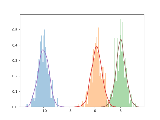
As a final step, let’s see how we did!

	import gmm
	out = gmm.fit(data, 3, 10, num_iter = 2000)
	sns.distplot(list(datapoints[0:333]), kde=False, bins=50, norm_hist=True)
	sns.distplot(list(datapoints[333:666]), kde=False, bins=50, norm_hist=True)
	sns.distplot(list(datapoints[666:]), kde=False, bins=50, norm_hist=True)
	sns.distplot(list(torch.distributions.Normal(loc=out[1][0], scale=1).sample((1000,))), kde=True, hist=False)
	sns.distplot(list(torch.distributions.Normal(loc=out[1][1], scale=1).sample((1000,))), kde=True, hist=False)
	sns.distplot(list(torch.distributions.Normal(loc=out[1][2], scale=1).sample((1000,))), kde=True, hist=False)
	plt.show()
	
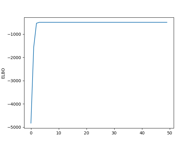
	plt.plot(list(out[3][0:100]))
	plt.ylabels("ELBO")
	plt.show()

Not bad! It looks like we converge relatively quickly and to a result that seems to be pretty reasonable.

To conclude, variational inference is a technique that approximates the posterior distribution using a parametric family of distributions. Fitting a model corresponds to finding the variational distribution that is closest to the true posterior, which we measure using the ELBO.

As a final remark, I’ll note that this algorithm still doesn’t quite scale that well. It is preferrable to MCMC for large datasets, since optimization problems will very frequently be faster than sampling problems, but as specified here, our VI algorithm still is unable to handle very large datasets of millions or billions of datapoints. This is something that I hope to address in the next post.